MACHINING CALCULATIONS

“Common sense is calculation applied to life.”
Henri-Frédéric Amiel

In addition to cutting data, machining calculations play a significant role in the strength and stiffness analysis of an entire technological system comprising a machine, a cutting tool, a clamping fixture, and a workpiece. The calculation results provide data regarding power consumption and cutting torque and form the initial foundation for designing new machines and fixtures. Additionally, the calculated material removal rate helps to understand the productivity of a cutting operation. Today, advanced computerized systems enable highly accurate calculations by considering various machining factors. However, quick and simplified calculations are often required. They help estimate the load on a cutting tool and other elements of the technological system. Moreover, they assist in verifying results obtained from computer software. This article discusses how to calculate material removal rate, cutting forces, and power consumption for machining operations.

Material removal rate (MRR) Q is a key indicator of machining productivity. The higher the Q, the more productive the machining. Material removal rate is the volume of material that is removed by tool per unit of time during machining operation. Calculating MRR depends on the machining process. Since metals have historically been the main engineering material, material removal rate is often referred to as “metal removal rate”.

For example, in turning
Q=vc×ap×f (1)
While in milling
Q=ap×ae×vf (2)

Here:
vc – cutting speed,
ap – depth of cut,
ae – width of cut,
f – feed (feed per revolution),
vf – feed speed (feed rate).

The MRR units are mm3/min or cm3/min in the metric system, and in3/min in the US customary (imperial) system. When calculating the metal removal rate, it is essential to ensure that the units of measurement for all variables in the equations are consistent. Mixing unsuitable units is not allowed, and it leads to wrong results. For example, in finding MRR using the values of depth and width of cut in mm (inches) together with cutting speed given in m/min (sfm) will cause serious error.
In drilling
Q=vc×ap×fz (3) where fz stands for feed per tooth.
For a drill in diameter d with z teeth (flutes), ap=d/2 and fz=f/z.
Hence
Q=vc×ap×fz=π×d×n×d/2×f/z=π×d2/(2×z)×n×f=π×d2/(2×z)×vf
Here n is the rotary velocity of a drill.
For typical two-flute drills z=2, and
Q=π×d2/4×vf (3a)

Example: Find the MRR for face milling operation performed using an ISCAR’s HELIDO shell mill with a diameter of 250 mm and 12 teeth, based on the data below:
depth of cut 5 mm
width of cut 180 mm
cutting speed 120 m/min
feed 0.25 mm/tooth
Rotary velocity of a milling cutter n=1000×vc/(π×d) =1000×120/(π×250) =153 (rpm)
Feed speed vf=fz×z×n =0.25×12×153=459 (mm/min)
Using equation (2):
Q=ap×ae×vf =5×180×459=413100 (mm3) =413.1 cm3

Example: A turning operation for 2.5” in Dia. bar is specified by 1000 rpm
spindle speed, 0.006 ipr feed and 0.08” depth of cut. Find MRR.
Cutting speed in sfm vc=π×d×n/12. Due to one foot comprises 12 inches, cutting speed in ipm is vc=π×d×n =π×2.5×1000=7854 (ipm).
Therefore, according to equation (1)
Q=vc×ap×f =7854×0.08×0.006=3.77 (in3)

So, the metal removal rate is an important machining characteristic that reflects cutting productivity. However, MRR cannot be considered isolated from other process parameters. One of them is tool life. There is no point in machining at such a high material removal rate causing the tool to break as soon as it starts cutting because of heavy loading caused by extreme cutting speeds and feeds. Another parameter relates to cutting power consumption.

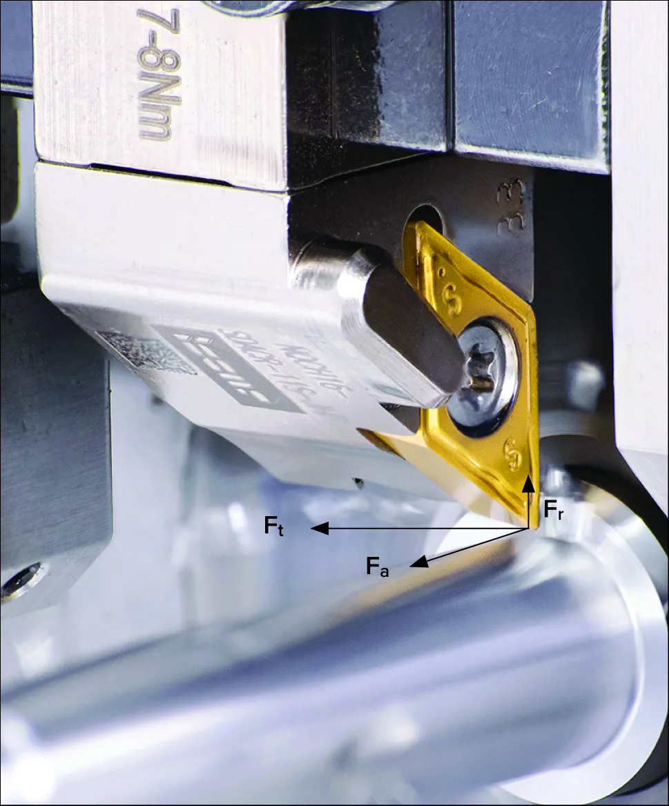
In cutting, the tool, which penetrates the material of a machined workpiece, is loaded by the material resistance force. This force is known as a resultant or total cutting force. The magnitude and the direction of this force depend on the machining process, the material machinability, cutting data, cutting conditions, and the tool cutting geometry. In the rectangular coordinate reference systems, a resultant (total) cutting force F can be resolved by three components:

tangential cutting force Ft
radial cutting force Fr
axial cutting force Fa
The word “cutting” in the description of cutting force components is often omitted.
Sometimes, the tangential, radial, and axial cutting forces are designated also as Fz, Fy, and Fx correspondingly.
F= √(〖Ft〗^2+〖Fr〗^2+〖Fa〗^2 ) (4)

Depending on the type of machining, the effect of the forces on the tool is different, and the magnitudes of these forces are in varying ratios with respect to each other. In machining with rotational mode of primary motion, tangential force Ft is the largest when compared to the other components. This force is considered the main cutting force component and determines the torque and power consumption required for cutting action. In turning (Fig. 1), radial force Fr, which is directed radially from the axis of rotation of a workpiece, pushes a turning tool away from the workpiece. The resulting pushing effect may be a source of vibrations that affect machining accuracy and surface finish. Axial force Fa that is directed longitudinally, parallel to the axis of rotation, acts against feed motion. In terms of turning, this force is also referred to as “longitudinal” force.

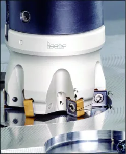
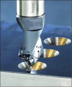
In milling (Fig. 2), radial force Fr, like in turning, pushes a milling cutter away from a workpiece. The resultant force Fb of Fr and Ft, which is called “bending force”, bends the cutter. The projection of this resultant force on the axis of feed motion forms the reaction force caused by a machine feed drive. Axial force Fa, acting along the cutter, loads the spindle unit bearings. In drilling (Fig. 3), axial force Fa corresponds to the main cutting edges (lips) of a drill. This force compresses a drill along the drill axis, and, together with force Fch acting on the drill chisel edge, establishes the power consumption of a feed drive.

Determining cutting forces is a key parameter in the design of machine tool units, work- and toolholding device, static and dynamic behavior of the cutting tool itself, and stiffness analysis of the entire technological system comprising machine, tool, fixtures, and the workpiece. The cutting forces are calculated by use of empirical equations. The more factors are taken into consideration in the equations, the more complicated these equations are. Another approach is based on the relationship between the cutting forces. As a function of the machining process, the cutting forces are related by a ratio to each other. The ratio looks like:
Ft:Fa:Fr=1:x:y (5)
Coefficients x and y depend on machining operations, machined material, cutting geometry and cutting material etc. In practice, using averaged values of x and y enables quite acceptable results. Therefore, after calculating tangential force Ft, the main component of the total cutting force, the other components can be easily found from equation (5). In estimating tangential force Ft, a method that is based on specific cutting force values is reasonable. In milling, for instance, the actual specific cutting force kc is the force that is needed to remove the material chip area of 1 mm2 (.0016 in2), which has an average chip thickness referred to as hm.
kc=kc1×hm-mc (6)
where kc1 is the specific cutting force to remove the material chip area of 1 mm2 (.0016 in2) with 1 mm (.004 in) thickness, mc is the chip thickness factor that reflects the dependence of kc on kc1 with changing the actual chip thickness when compared to 1 mm2 (.0016 in2). kc1 and mc are characteristics of the machined material based on test results. The analysis of empirical data has enabled specifying these characteristics as averaged values for all groups of engineering materials. In various sources of machining data, kc1 relates to cutting material with a tool bearing a zero rake angle (γ=0°). If the actual tool rake significantly differs from zero, the above equation may be corrected in the following way:
kc=kc1×hm-mc×(1-γ/100) (7)
Knowing the specific force and the cross-section area of the cut material layer A, one can easily determine the tangential force.
Example: A 90-degree milling cutter machines a square shoulder that has cross-sectional dimensions 4 mm×9.5 mm (.16”×.38”). The workpiece material is annealed high alloyed steel AISI H13 (DIN W.-Nr. 1.2344). The rake angle of the cutter is 10°. We need to find the tangential cutting force if 0.1 mm average chip thickness (.004” chip load) is maintained.

According to the Materials and Grade section in ISCAR’s Milling Line Catalog, the machined material relates to a material group, which features
kc1 =2450 N/mm2 (355 ksi) and mc=0.23.
From equation (7) actual cutting force
kc=2450×0.1-0.23× (1-0.1) = 3745 N/mm2 (543166 psi or ~543 ksi).
Tangential cutting force
Ft’= 3745×4×9.5 = 142310 N= 142.3 kN,
and Ft’’= 543166×0.16×0.3 8= 33024 lbf (~33 klbf).
Determining the tangential cutting force enables finding cutting power consumption P and, consequently, the estimated power required at the main drive of a machine tool. P=Ft×vf=A×kc×vf (9)
If a and b are the depth and the width of a cut layer cross-section A, then consider the following unit conversion:
in metric system
P=(a×b×kc×vf) / (6×107) kW (10a)
where a and b in mm, kc in N/mm2 and vf in mm/min
in the US customary (imperial) system
P=(a×b×kc×vf) / (12×33000)=(a×b×kc×vf)/396000 hp (10b)
where a and b in inches, kc in psi and vf in ipm
If kc is given in ksi, the numerical coefficient of unit conversion in the
denominator of the above equation is reduced one thousand times:
P=(a×b×kc×vf) / (12×33) =(a×b×kc×vf)/396 hp (10c)

Example: Let’s go back to the previous example and find the cutting power consumption if the cutter has 4 flutes and 16 mm (.625”) diameter, and the machining features a cutting speed of 120 mm/min (394 sfm) and a feed per tooth 0.1 mm/tooth (.004 ipt).
Spindle speed n is calculated as following:
n’=(1000×vc)/(π×d) in metric units and
n’’=(12× vc)/(π×d) in US customary (imperial) units.
Hence, n’=(1000×120)/(π×16) =2387 (rpm) and
n’’=(12×394)/(π×0.625) =2408 (rpm).
Correspondingly, feed speed vf=fz×z×n:
vf’=0.1×4×2387=954.8 (mm/min)
vf’’=0.004×4×2408=38.53 (ipm)
According to equation (10a) and (10c):
P’=(142310×954.8) / (6×107) =2.26 (kW)
P’’=(0.16×0.38×543×38.53) / 396 =3.21 (hp)

Computerization of metal cutting has opened new prospects for accurate engineering calculations. Advanced software enables realizing complicated empirical models which emerge new levels of calculations. ISCAR’s Machining Power Calculator estimates power consumption, cutting forces, bending moment, load time variations, plot charts and other important parameters during machining. The Calculator is available for PC and mobile applications.